
Hebbian Learning is one of the most famous learning theories. It was proposed by the Canadian psychologist Donald Hebb in 1949, many years before his results were confirmed through neuroscientific experiments. Artificial Intelligence researchers immediately understood the importance of his theory when applied to artificial neural networks, and even if more efficient algorithms have been adopted in order to solve complex problems, neuroscience continues finding more and more evidence of natural neurons whose learning process is almost perfectly modeled by Hebb’s equations.
Hebb’s rule is very simple and can be discussed starting from a high-level structure of a neuron with a single output:

We are considering a linear neuron; therefore, the output y is a linear combination of its input values x:

According to the Hebbian theory, the corresponding synaptic weight will be reinforced if both pre and post-synaptic units behave similarly (firing or remaining steady). On the other hand, if their behavior is discordant, we will be weakened. In other words, using a famous aphorism, “Neurons that fire together, wire together.” From a mathematical viewpoint, this rule can expressed (in a discretized version) as:

Alpha is the learning rate. To better understand the implications of this rule, it’s useful to express it using vectors:

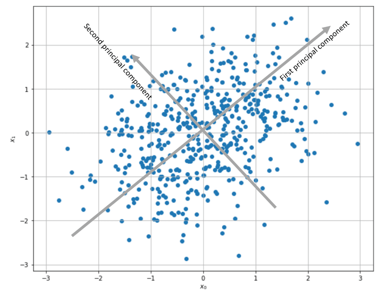
C is the input correlation matrix (if the samples are zero-centered, C is also the covariance matrix). Therefore, the weight vector will be updated to maximize the components corresponding to the input maximum variance direction. In particular, considering the time-continuous version, if C has a dominant eigenvalue, the solution w(t) can be expressed as a vector with the same direction as the corresponding C eigenvector. In other words, Hebbian learning performs a PCA, extracting the first principal component.
Even if this approach is feasible, this rule has a problem: it is unstable. C is a positive semidefinite matrix. Therefore, its eigenvalues are always non-negative. That means the w(t) will be a linear combination of eigenvectors with coefficients increasing exponentially with t. Considering the discrete version, it’s easy to understand that if x and y are greater than 1, the learning process will indefinitely increase the absolute value of the weights, producing an overflow.
This problem can be solved by imposing the normalization of weights after each update (so as to make them saturate to finite values). Still, this solution is biologically unlikely because each synapse needs to know all other weights. Oja has proposed the best alternative approach, and the rule is named after him:

The rule is always Hebbian but now includes an auto-normalizing term (-wy²). It’s easy to show the corresponding time-continuous differential equation now has negative eigenvalues, and the solution w(t) converges. Just like in the pure Hebb’s rule, the vector w will always converge to the dominant C eigenvector, but in this case, its norm will be a finite (small) number.
Implementing Oja’s rule in Python (with Tensorflow, too) is very easy. Let’s start with a random bidimensional centered dataset (obtained using Scikit-Learn make_blobs() and StandardScaler()):
In the following GIST, the covariance (correlation) matrix is computed, together with its eigenvectors, and then Oja’s rule is applied to the dataset:
import numpy as np

from sklearn.datasets import make_blobs
from sklearn.preprocessing import StandardScaler

# Set random seed for reproducibility
np.random.seed(1000)

# Create and scale dataset
X, _ = make_blobs(n_samples=500, centers=2, cluster_std=5.0, random_state=1000)

scaler = StandardScaler(with_std=False)
Xs = scaler.fit_transform(X)

# Compute eigenvalues and eigenvectors
Q = np.cov(Xs.T)
eigu, eigv = np.linalg.eig(Q)

# Apply the Oja's rule
W_oja = np.random.normal(scale=0.25, size=(2, 1))
prev_W_oja = np.ones((2, 1))

learning_rate = 0.0001
tolerance = 1e-8

while np.linalg.norm(prev_W_oja - W_oja) > tolerance:
    prev_W_oja = W_oja.copy()

    Ys = np.dot(Xs, W_oja)
    W_oja += learning_rate * np.sum(Ys*Xs - np.square(Ys)*W_oja.T, axis=0).reshape((2, 1))
# Eigenvalues
print(eigu)

[ 0.67152209  1.33248593]

# Eigenvectors
print(eigv)

[[-0.70710678 -0.70710678]
 [ 0.70710678 -0.70710678]]

 # W_oja at the end of the training process
 print(W_oja)

 [[-0.70710658]
 [-0.70710699]]
As it’s possible to observe, the algorithm has converged to the second eigenvector, whose corresponding eigenvalue is the highest.
An extension to the Oja’s rule to multi-output networks is provided by the Sanger’s rule (also known as Generalized Hebbian Algorithm):

In this case, the normalizing (and decorrelating) factor is applied, considering only the synaptic weights before the current one (included). Using a vectorial notation, the update rule becomes:

Tril() is a function that returns the lower triangle of a square matrix. Sanger’s rule can extract all principal components, starting from the first and continuing with all output units. Just like for Oja’s rule, in the following GIST, the rule is applied to the same dataset:
import numpy as np

from sklearn.datasets import make_blobs
from sklearn.preprocessing import StandardScaler

# Set random seed for reproducibility
np.random.seed(1000)

# Create and scale dataset
X, _ = make_blobs(n_samples=500, centers=2, cluster_std=5.0, random_state=1000)

scaler = StandardScaler(with_std=False)
Xs = scaler.fit_transform(X)

# Compute eigenvalues and eigenvectors
Q = np.cov(Xs.T)
eigu, eigv = np.linalg.eig(Q)

W_sanger = np.random.normal(scale=0.1, size=(2, 2))
prev_W_sanger = np.ones((2, 2))

learning_rate = 0.1
nb_iterations = 2000
t = 0.0

for i in range(nb_iterations):
    prev_W_sanger = W_sanger.copy()
    dw = np.zeros((2, 2))
    t += 1.0

    for j in range(Xs.shape[0]):
        Ysj = np.dot(W_sanger, Xs[j]).reshape((2, 1))
        QYd = np.tril(np.dot(Ysj, Ysj.T))
        dw += np.dot(Ysj, Xs[j].reshape((1, 2))) - np.dot(QYd, W_sanger)

    W_sanger += (learning_rate / t) * dw
    W_sanger /= np.linalg.norm(W_sanger, axis=1).reshape((2, 1))
# Eigenvalues
print(eigu)

[ 0.67152209  1.33248593]

# Eigenvectors
print(eigv)

[[-0.70710678 -0.70710678]
 [ 0.70710678 -0.70710678]]

# W_sanger at the end of the training process
print(W_sanger)

[[-0.72730535 -0.69957863]
 [-0.67330094  0.72730532]]
As it’s possible to observe, the weight matrix contains (as columns) the two principal components (roughly parallel to the eigenvectors of C).
Thanks to its simplicity and biological evidence, Hebbian learning is a potent, unsupervised approach. Applying this methodology to bio-inspired problems like orientation sensitivity is easy. I recommend [1] for further details about these techniques and other neuroscientific models.
References:
-
- Dayan P., Abbott L. F., Theoretical Neuroscience: Computational and Mathematical Modeling of Neural Systems, The MIT Press
If you like this post, you can always donate to support my activity! One coffee is enough!