Contrary to most machine learning algorithms, Instance-Based Learning is model-free, meaning there are strong assumptions about the structure of regressors, classifiers, or clustering functions. They are “simply” determined by the data, according to an affinity induced by a distance metric (the most common name for this approach is Nearest Neighbors).
If we have a dataset X:

it’s possible to introduce a metric in the m-dimensional hyperspace. The most common choice is the Euclidean metric:
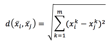
Computing the distance between every couple of samples, we get a symmetric matrix, which is already a global measure of the affinity among points:

Indeed, even if it’s not a model, this is the most similar thing to a model based on the natural structure of the training data. Considering that the hyperspace is normally a feature space; two points that are close share (or have similar) features. This is the only real assumption in this kind of approach, and, in fact, the geometry of the dataset (together with a distance function) is the algorithm itself. Therefore, a prediction is made by searching to the top k nearest neighbors and:
-
- In a clustering approach, consider them as a set of very similar objects whose features can be inherited by the new sample. A common application is in user-based recommendation systems, where a new user has to “borrow” the features provided by his/her neighbors.
- In a classification approach, averaging the classes (it’s also possible to weight them using the normalized distances), it’s easy to determine the class of the new sample.
- In a regression approach, considering the weighted value of all neighbors as training points for a standard regression
Unfortunately, computing M is very expensive; with n samples belonging to an m-dimensional space, we need to compute m multiplications for every couple of samples. It means that this algorithm, often called “brute-force” has a “training” complexity O(mn²) and a prediction complexity O(mn), showing to suffer a dramatic curse of dimensionality.
To overcome this problem, two alternatives have been proposed (and they are all implemented by Scikit-Learn):
-
- KD-Trees
- Ball-Trees
A KD tree is a natural extension of a binary tree to K-dimensional data. The idea is quite simple and can be explained considering the following figure:
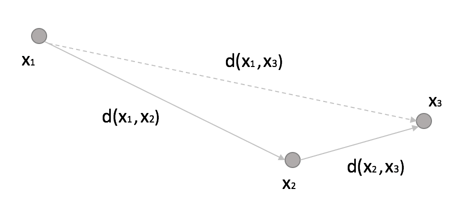
If we set a threshold R, then:

In other words, if the distance between x1 and x2 overcomes a fixed threshold (disqualifying x2 from being a neighbor) and the distance between x2 and x3 is much shorter than R, then x3 is also a non-neighbor, and it doesn’t make sense to compute the distance between x1 and x3 explicitly. With a KD-Tree, the space is partitioned using binary k-dimensional nodes, and in each of them, only a single dimension is chosen to split the original sub-space into two half-spaces. The dynamic is very intuitive in 2D. Thanks to Wikipedia contributors KiwiSunset and MYguel, I can show a simple example without the need to redraw from scratch.
There are 6 points in a 2D space:
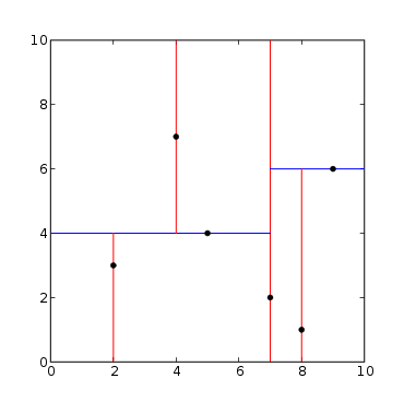
The red lines represent cuts on the X-axis and the red lines on the Y-axis. Starting from the point (7, 2) and cutting on X, we have 3 points where x<7 and two points where x>7:
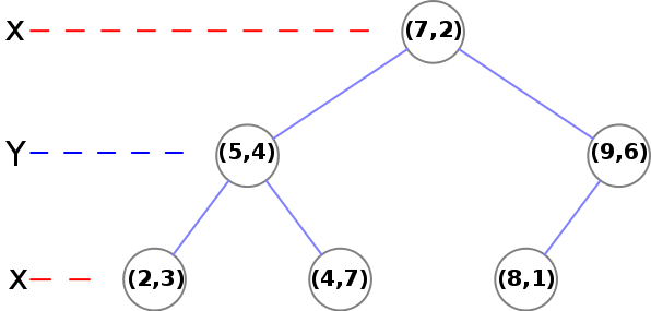
At the second level, we need to use Y:
-
- (5, 4) -> There is one node (2, 3) where y<4 and another node (4, 7) where y>4
- (9, 6) -> There is a final (leaf) node (8, 1)
The procedure is simple and can be extended to k-dimensional samples. As it is a binary tree, the training complexity becomes O(mn log(n)). Even if this is a better result than a brute-force algorithm, a KD-Tree isn’t able to exploit the radial structure of the Euclidean metric, and it’s very sensitive to the dimensionality.
Ball-Tree represents an alternative algorithm that can often outperform KD-Tree. A ball tree is always a binary tree, but, in this case, each node defines a hypersphere, and two sub-nodes define two sub-hyper-spheres whose union must contain all points assigned to the parent node, and whose intersection is always empty (even if the hyperspheres overlap). The dynamic is not very different from KD-Trees, but in general, Ball-Trees are more efficient when the dimensionality is very high. In fact, considering a scenario similar to the one previously presented, we can consider a point x1 (possibly a prediction point) and another point x2 with a subtree where we find x3 and x4:
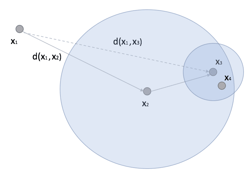
In research, if x2 is the closest point (to x1), then all the points belonging to the ball whose centroid has a distance from x1 greater than d(x1, x2) can be completely discarded because all its points are more distant than x2. If the ball is very dense, it dramatically reduces the number of comparisons, and the overall performance becomes superior to the version with KD-Tree.
Scikit-Learn implements clustering, classification, and regression based on k-Nearest-Neighbors algorithms (with brute-force, KD-Trees, Ball-Trees, and different metrics). Usage is very intuitive, and there’s no need to provide further examples (on the website, there are many interesting applications). However, I wanted to benchmark the performances of all algorithms. In the following snippet, 10 datasets (with an increasing number of samples and dimensions) are created, and a NearestNeighbors instance is initialized for each couple (dataset, algorithm):
from sklearn.datasets import make_blobs
from sklearn.neighbors import NearestNeighbors

import matplotlib.pyplot as plt
import multiprocessing
import numpy as np
import time

# Set random seed (for reproducibility)
np.random.seed(1000)

nb_samples = [50, 100, 500, 1000, 2000, 5000, 10000, 50000, 100000, 500000]
nb_features = [10, 25, 50, 75, 100, 150, 250, 300, 400, 500, 800, 1000, 2000]

algorithms = ['brute', 'kd_tree', 'ball_tree']

training_times = {'brute': [],
                  'kd_tree': [],
                  'ball_tree': []}

prediction_times = {'brute': [],
                    'kd_tree': [],
                    'ball_tree': []}

for i in range(len(nb_samples)):
    for algorithm in algorithms:
        X, _ = make_blobs(n_samples=nb_samples[i], n_features=nb_features[i],
                          centers=int(nb_features[i]/10), random_state=1000)

        # Create k-Nearest Neighbors instance
        nn = NearestNeighbors(algorithm=algorithm, n_jobs=multiprocessing.cpu_count())

        # Training
        start_time = time.time()
        nn.fit(X)
        end_time = time.time()

        training_times[algorithm].append(end_time - start_time)

        # Prediction
        xs = np.random.uniform(-1.0, 1.0, size=nb_features[i])

        start_time = time.time()
        nn.kneighbors(xs.reshape(1, -1), n_neighbors=5)
        end_time = time.time()

        prediction_times[algorithm].append(end_time - start_time)

# Show the results
fig, ax = plt.subplots(6, 1, figsize=(12, 17))

# Training times
ax[0].set_title('Training time (Brute-force algorithm)')
ax[0].set_xlabel('Number of samples')
ax[0].set_ylabel('Time (seconds)')
ax[0].plot(nb_samples, training_times['brute'])
ax[0].grid()

ax[1].set_title('Training time (KD-Tree algorithm)')
ax[1].set_xlabel('Number of samples')
ax[1].set_ylabel('Time (seconds)')
ax[1].plot(nb_samples, training_times['kd_tree'])
ax[1].grid()

ax[2].set_title('Training time (Ball-Tree algorithm)')
ax[2].set_xlabel('Number of samples')
ax[2].set_ylabel('Time (seconds)')
ax[2].plot(nb_samples, training_times['ball_tree'])
ax[2].grid()

# Prediction times
ax[3].set_title('Prediction time (Brute-force algorithm)')
ax[3].set_xlabel('Number of samples')
ax[3].set_ylabel('Time (seconds)')
ax[3].plot(nb_samples, prediction_times['brute'])
ax[3].grid()

ax[4].set_title('Prediction time (KD-Tree algorithm)')
ax[4].set_xlabel('Number of samples')
ax[4].set_ylabel('Time (seconds)')
ax[4].plot(nb_samples, prediction_times['kd_tree'])
ax[4].grid()

ax[5].set_title('Prediction time (Ball-Tree algorithm)')
ax[5].set_xlabel('Number of samples')
ax[5].set_ylabel('Time (seconds)')
ax[5].plot(nb_samples, prediction_times['ball_tree'])
ax[5].grid()

plt.show()
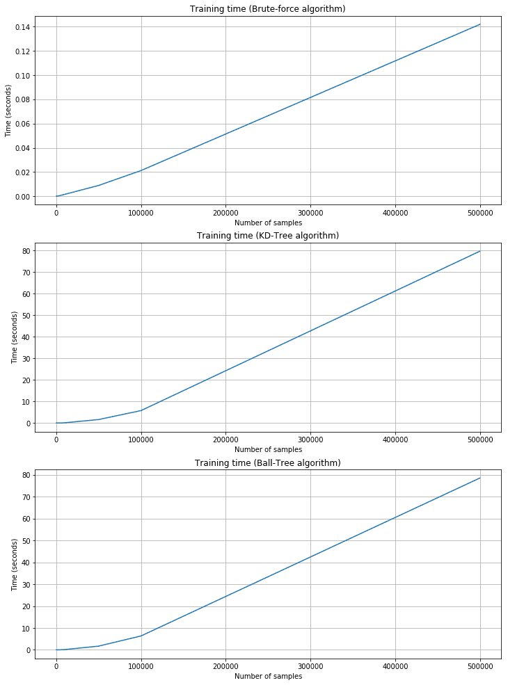
Training time plots:
Prediction time plots:
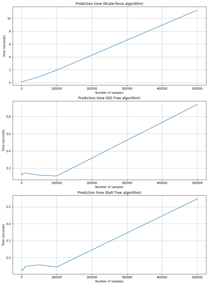
As expected, the training time is shorter for brute force, but the corresponding prediction time is quite longer. KD-Tree and Ball-Tree have longer training times due to the need to build the trees. However, queries are very fast. For example, with 500,000 2000-dimensional samples, the brute force needs about 11 seconds, while KD-Tree is about 0.95 and Ball-Tree is 0.55. Brute force performances are acceptable only when n and m are very small and the cost of building a tree is too high. In all those cases, Scikit-Learn provides a fourth alternative called ‘auto,’ which automatically selects the best strategy according to the dimensionality and uses ‘leaf_size’ to pass from a tree-based algorithm to the brute-force one.
If you like this post, you can always donate to support my activity! One coffee is enough!

