
Fisher Information, named after the statistician Ronald Fisher, is a powerful Bayesian Statistics and Machine Learning tool. To understand its “philosophical” meaning, it’s useful to think about a simple classification task, where our task is to find a model (characterized by a set of parameters) that is able to reproduce the data-generating process p(x) (normally represented as a data set) with the highest possible accuracy. This condition can be expressed using the Kullback-Leibler divergence:
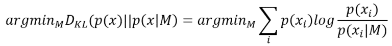
Finding the best parameters that minimize the Kullback-Leibler divergence is equivalent to maximizing the log-likelihood log P(x|M) because p(x) doesn’t contain any reference to M. Now, a good (informal) question is: how much information p(x) can provide to simplify the task to the model? In other words, given a log-likelihood, which is its behavior next to the MLE point?
Considering the following two plots, we can observe two different situations. The first is a very peaked likelihood, where the probability of any parameter value far from the MLE is almost near zero. In the second chart, the curve is flatter, and p(MLE) is very close to many sub-optimal states.
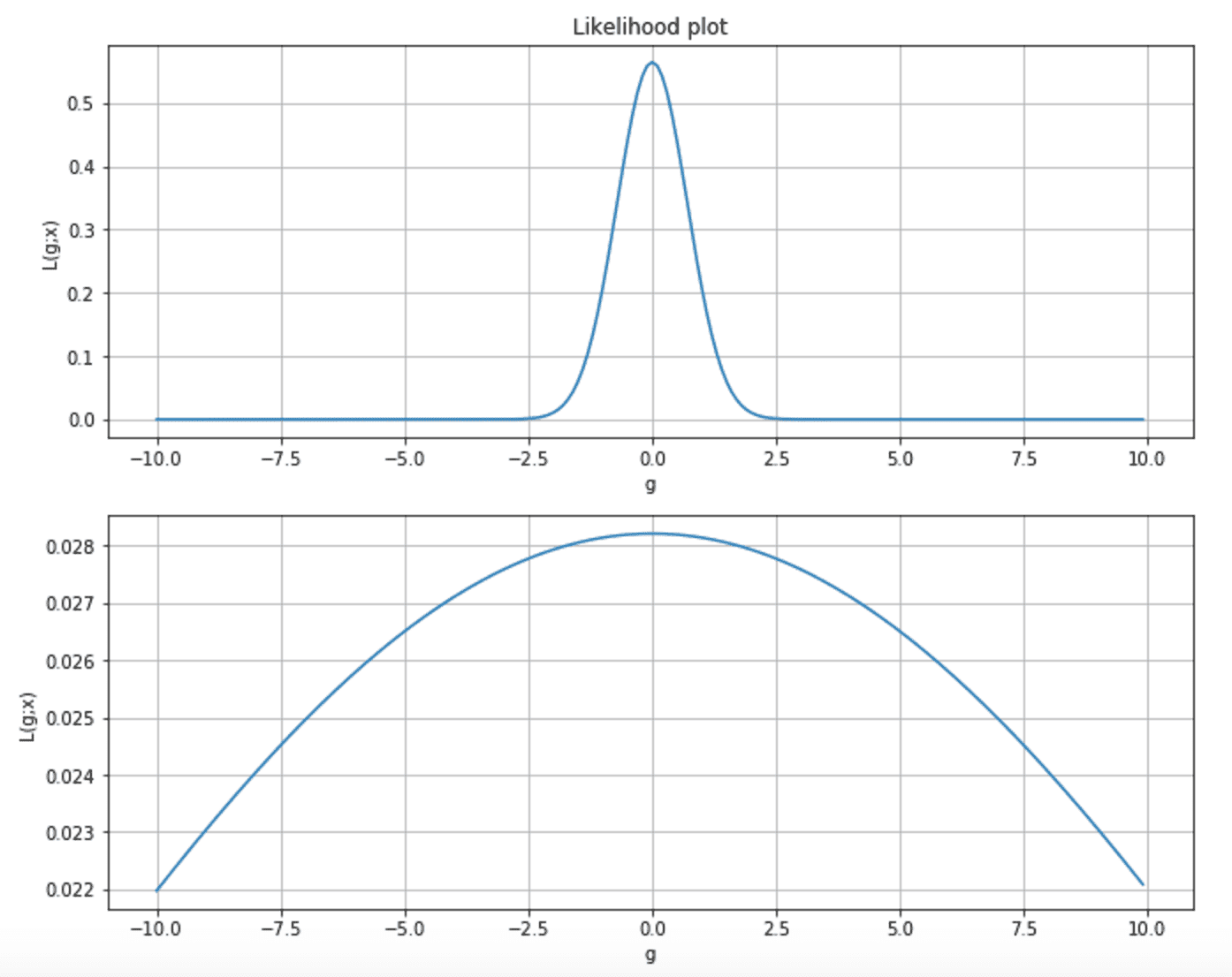
Moreover, as the majority of learning techniques rely on the gradient, in the first case, its magnitude is very when getting close to the MLE, while, in the second, the speed of the gradient is very slow, and the learning process can take a quite long time to reach the maximum.
Fisher Information helps determine how much peaked the likelihood function is and provides a precise measure of the amount of information that the data generating process p(x) can supply to M to reach the MLE. The simplest definition is based on a single parameter ρ. In a discrete form (more common in machine learning), it’s equivalent to:
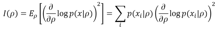
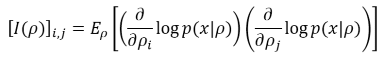
The lower bound is 0, meaning no information is provided, while there’s no upper bound (+∞). If the model, as often happens, has many parameters (ρ1, ρ2, …, ρN), it’s possible to compute the Fisher Information Matrix, defined as:
Under some regularity conditions, it’s possible to transform both expressions using second derivatives (very often, the Fisher Information Matrix) is computed as negative Hessian). However, I prefer to keep the original expressions because they can always be applied without particular restrictions. Even if, without explicit second derivatives, the Fisher Information provides a “speed” of the gradient computed for each parameter. The faster it is, the easier the learning process.
Now, let’s suppose that we are estimating the value of a parameter ρ, through an approximation ρ′. If E[ρ′] = ρ, the estimator is called unbiased, and the only statistical element to consider is the variance. If the expected value is correct, but the variance is very high, the probability of a wrong value is also very high. Therefore, in machine learning, we’re interested in knowing the minimum variance of an unbiased estimator. The Cramér-Rao bound states that:
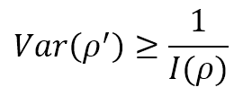
Therefore, high Fisher Information implies a lower bound variance, while low Fisher Information limits our model by imposing a high minimum achievable variance. Of course, this doesn’t mean that every unbiased estimator can reach the Cramér-Rao bound. Still, it provides us with a measure of the theoretical maximum accuracy we can achieve if our model is powerful enough.
To show how to compute the Fisher Information Matrix and apply the Cramér-Rao bound, let’s consider a very simple dataset (our data-generating process) that a Logistic Regression can easily learn:
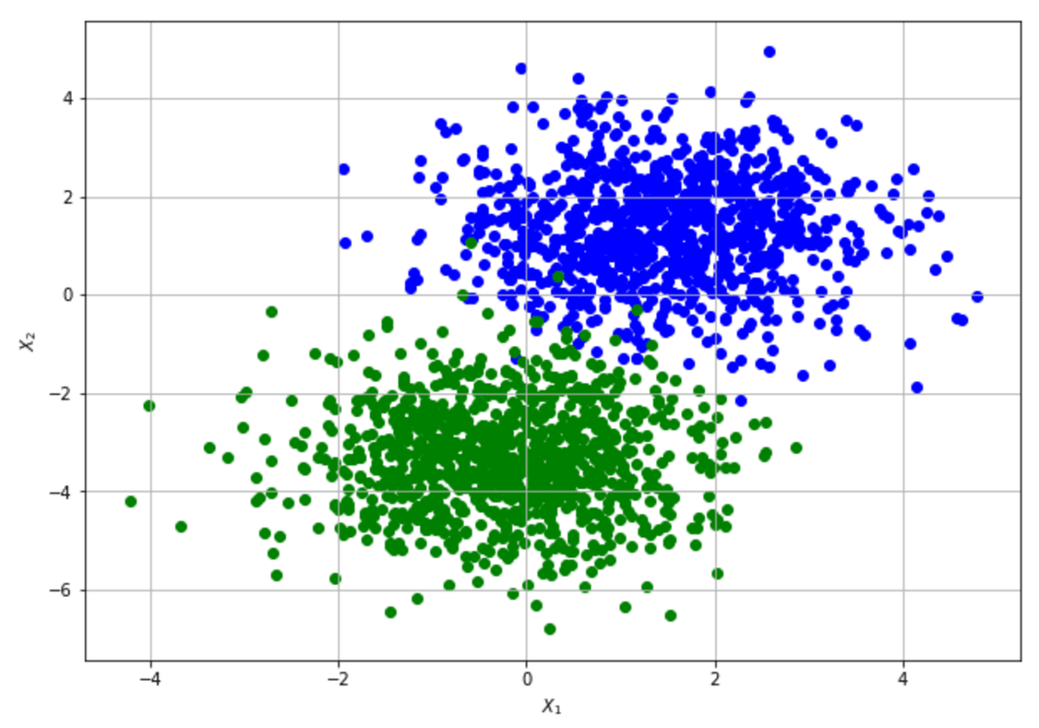
For the sake of simplicity, the 2D data set has been modified by adding a “ones” column to learn the bias as any other weight. The implementation is based on Tensorflow (available on this GIST), which allows numerically stable gradient computation:
import numpy as np
import tensorflow as tf

from sklearn.datasets import make_blobs

# Set random seed (for reproducibility)
np.random.seed(1000)

# Create dataset
nb_samples=2000
X, Y = make_blobs(n_samples=nb_samples, n_features=2, centers=2, cluster_std=1.1, random_state=2000)

# Transform the original dataset so to learn the bias as any other parameter
Xc = np.ones((nb_samples, X.shape[1] + 1), dtype=np.float32)
Yc = np.zeros((nb_samples, 1), dtype=np.float32)

Xc[:, 1:3] = X
Yc[:, 0] = Y

# Create Tensorflow graph
graph = tf.Graph()

with graph.as_default():
    Xi = tf.placeholder(tf.float32, Xc.shape)
    Yi = tf.placeholder(tf.float32, Yc.shape)

    # Weights (+ bias)
    W = tf.Variable(tf.random_normal([Xc.shape[1], 1], 0.0, 0.01))

    # Z = wx + b
    Z = tf.matmul(Xi, W)

    # Log-likelihood
    log_likelihood = tf.reduce_sum(tf.nn.sigmoid_cross_entropy_with_logits(logits=Z, labels=Yi))

    # Cost function (Log-likelihood + L2 penalty)
    cost = log_likelihood + 0.5*tf.norm(W, ord=2)

    trainer = tf.train.GradientDescentOptimizer(0.000025)
    training_step = trainer.minimize(cost)

    # Compute the FIM
    dW = tf.gradients(-log_likelihood, W)
    FIM = tf.matmul(tf.reshape(dW, (Xc.shape[1], 1)), tf.reshape(dW, (Xc.shape[1], 1)), transpose_b=True)

# Create Tensorflow session
session = tf.InteractiveSession(graph=graph)

# Initialize all variables
tf.global_variables_initializer().run()

# Run a training cycle
# The model is quite simple, however a check on the cost function should be performed
for _ in range(3500):
    _, _ = session.run([training_step, cost], feed_dict={Xi: Xc, Yi: Yc})

# Compute Fisher Information Matrix on MLE
fisher_information_matrix = session.run([FIM], feed_dict={Xi: Xc, Yi: Yc})
The resulting Fisher Information Matrix is:
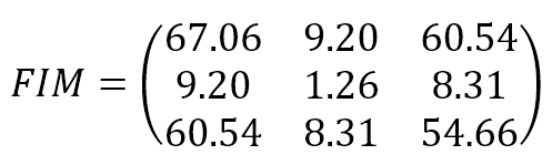
The parameters are (bias, w1, w2). The result shows that the original data set provides relatively high information when estimating the bias and w2 and lower information when estimating w1. The Cramér-Rao bound sets a minimum variance for bias and w2 and a relatively higher value for w1. The structure of the data set can derive an interpretation of this result: moving along the x2 axis, it’s easy to find a boundary that separates blue and green dots; on the other hand, this is not true when exploring the first dimension. Conversely, none of the FIM values are 0 (or very close to 0), meaning that the parameters aren’t orthogonal and can’t be learned separately.
If you want to obtain an analytic FIM expression, it’s necessary to consider all possible (or a broad set) values and compute the expected value averaging over ρ.
For a deeper understanding of Fisher Information, you can see this lecture on YouTube:

If you like this post, you can always donate to support my activity! One coffee is enough!