Quickprop: an almost forgotten neural training algorithm

Standard Back-propagation is probably the best neural training algorithm for shallow and deep networks. However, it is based on the chain rule of derivatives, and an update in the first layers requires knowledge back-propagated from the last layer. This non-locality, especially in deep neural networks, reduces the biological plausibility of the model because, even if there’s enough evidence of negative feedback in real neurons, it’s unlikely that, for example, synapsis in LGN (Lateral Geniculate Nucleus) could change their dynamics (weights) considering a chain of changes starting from the primary visual cortex. Moreover, classical back-propagation doesn’t scale very well in large networks.

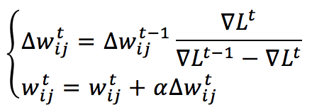
For these reasons, in 1988, Fahlman proposed an alternative local and quicker update rule, where the total loss function L is approximated with a quadratic polynomial function (using Taylor expansion) for each weight independently (assuming that each update has a limited influence on the neighbors). The resulting weight update rule (which is a pseudo-second-order method) is:

L is the cost function (total loss function), and the gradient must be computed according to the connection between neuron i (belonging to a higher layer) and neuron j (belonging to a lower layer): ∇L(i,j), while alpha is the learning rate. This rule is completely local (because it depends only on the information gathered from the pre and post-synaptic units) and can also be very fast when the problem is convex but, on the other side, has some heavy drawbacks:

• • It needs to store the previous gradient and weight correction (this is partially biologically plausible)
  • It can produce “uncertain” jumps when the error surface has many local minima due to the approximation of the loss function and its second derivative

For these reasons, this algorithm has been almost abandoned in favor of Back-propagation that, together with the most common optimizers, like RMSProp or Adam, can reach the convergence in very deep networks without particular drawbacks.

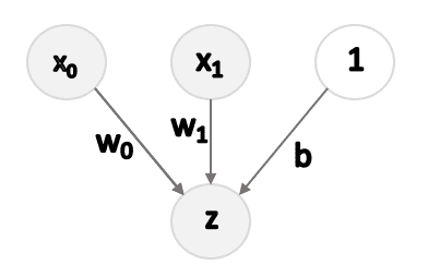
To test Quickprop, I’ve implemented a very simple neural network (actually a Logistic Regression):

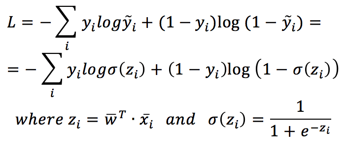
For simplicity, the X dataset has been transformed into a (N, 3) matrix, with the third column equal to 1. In this way, the bias can be learned just like any other weight. The cost function based on the cross-entropy is:

The generic gradient (in this case, I’ve considered only a single index because there’s only one layer) is:

The full code is also available in the GIST:

from sklearn.datasets import make_classification

import numpy as np

# Set random seed (for reproducibility)
np.random.seed(1000)

def sigmoid(arg):
    return 1.0 / (1.0 + np.exp(-arg))

# Create random dataset
nb_samples = 500
nb_features = 2

X, Y = make_classification(n_samples=nb_samples, 
                           n_features=nb_features, 
                           n_informative=nb_features, 
                           n_redundant=0, 
                           random_state=4)

# Prepreprocess the dataset
Xt = np.ones(shape=(nb_samples, nb_features+1))
Xt[:, 0:2] = X
Yt = Y.reshape((nb_samples, 1))

# Initial values
W = np.random.uniform(-0.01, 0.01, size=(1, nb_features+1))
dL = np.zeros((1, nb_features + 1))
dL_prev = np.random.uniform(-0.001, 0.001, size=(1, nb_features + 1))
dW_prec = np.ones((1, nb_features + 1))
W_prev = np.zeros((1, nb_features + 1))

learning_rate = 0.0001
tolerance = 1e-6

# Run a training process
i = 0

while np.linalg.norm(W_prev - W, ord=1) > tolerance:
    i += 1
    
    sZ = sigmoid(np.dot(Xt, W.T))
    
    dL = np.sum((Yt - sZ) * Xt, axis=0)
    delta = dL / (dL_prev - dL)
    dL_prev = dL.copy()
    
    dW = dW_prec * delta
    dW_prec = dW.copy()
    
    W_prev = W.copy()
    W += learning_rate * dW
    
print('Converged after {} iterations'.format(i))

The complexity is very limited, but it’s possible to see that Quickprop can converge very quickly. In the case of oscillations, it’s better to reduce the learning rate (this slows down the overall speed, too). However, in general, for every problem when Quickprop has to be employed, it’s useful to find the optimal hyperparameters (learning rate and number of iterations).

For further details:

• • Fahlman S. E., An Empirical Study of Learning Speed in Back-Propagation Networks
  • Rojas R., Neural Networks: A Systematic Introduction, Springer

---

If you like this post, you can always donate to support my activity! One coffee is enough!

---