
One of the most interesting effects of PCA (Principal Component Analysis) is to decorrelate the input covariance matrix C by computing the eigenvectors and operating a base change using a matrix V:
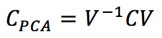
The eigenvectors are sorted in descending order, considering the corresponding eigenvalue. Therefore, Cpca is a diagonal matrix where the non-null elements are λ1 >= λ2 >= λ3 >= … >= λn. By selecting the top p eigenvalues, it’s possible to operate a dimensionality reduction by projecting the samples in the new sub-space determined by the p top eigenvectors (it’s possible to use Gram-Schmidt orthonormalization if they don’t have a unitary length). The standard PCA procedure works with a bottom-up approach, obtaining the decorrelation of C as a final effect. However, it’s possible to employ neural networks, imposing this condition as an optimization step. One of the most influential models has been proposed by Rubner and Tavan (and it’s named after them). Its generic structure is:
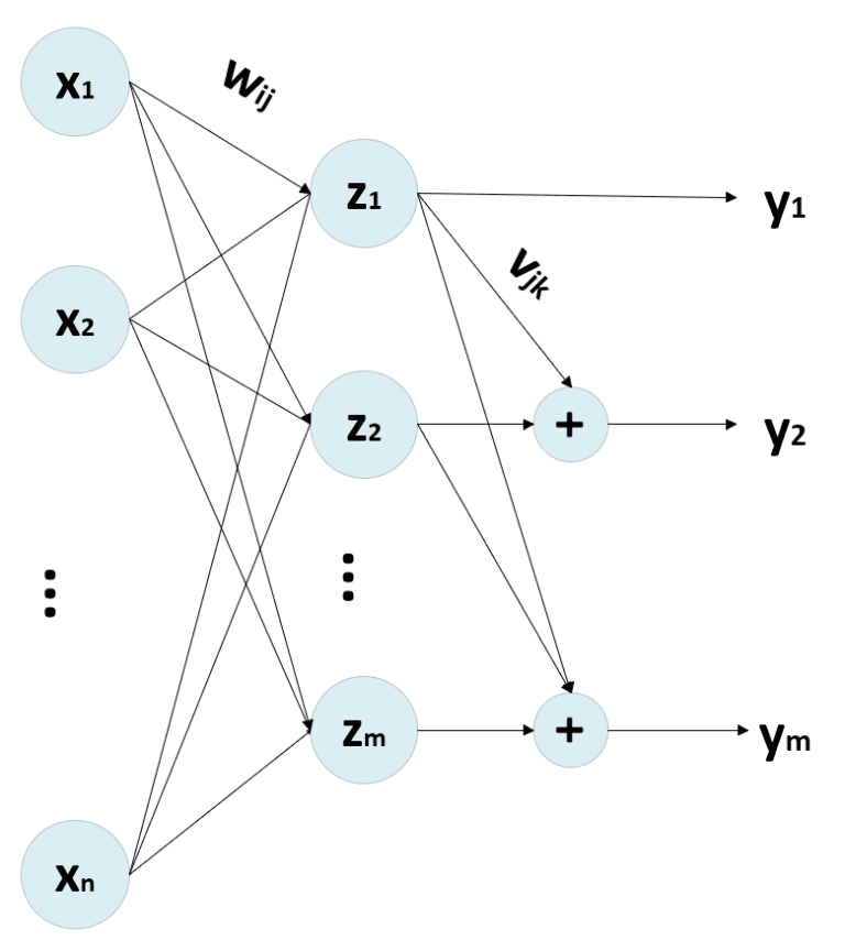
Where we suppose that N (input-dimensionality) << M (output-dimensionality), the output of the network can be computed as:
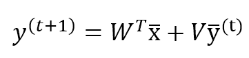
Where V (n × n) is a lower-triangular matrix with all diagonal elements to 0, and W has a shape (n × m). Moreover, it’s necessary to store the y(t) to compute y(t+1). This procedure must be repeated until the output vector has been stabilized. Generally, after k < 10 iterations, the modifications are under a threshold of 0.0001. However, it’s important to check this value in every real application.
The training process is managed with two update rules:
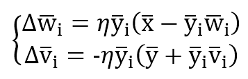
The first one is Hebbian based on Oja’s rule, while the second is anti-Hebbian because its purpose is to reduce the correlation between output units. In fact, without the normalization factor, the update is in the form dW = -αy(i)y(k) to reduce the synaptic weight when two output units are correlated (same sign).
If the matrix V is kept upper-triangular, it’s possible to vectorize the process. There are also other variants, like the Földiák network, which adopts a symmetric V matrix to add the contribution of all other units to y(i). However, the Rubner-Tavan model seems more similar to the process adopted in a sequential PCA, where the second component is computed as orthogonal to the first and so forth until the last one.
The example code is based on the MNIST dataset provided by Scikit-Learn and adopts a fixed number of cycles to stabilize the output. The code is also available in this GIST:
from sklearn.datasets import load_digits

import numpy as np

# Set random seed for reproducibility
np.random.seed(1000)

# Load MNIST dataset
X, Y = load_digits(return_X_y=True)
X /= 255.0

n_components = 16
learning_rate = 0.001
epochs = 20
stabilization_cycles = 5

# Weight matrices
W = np.random.uniform(-0.01, 0.01, size=(X.shape[1], n_components))
V = np.triu(np.random.uniform(-0.01, 0.01, size=(n_components, n_components)))
np.fill_diagonal(V, 0.0)

# Training process
for e in range(epochs):
    for i in range(X.shape[0]):
        y_p = np.zeros((n_components, 1))
        xi = np.expand_dims(Xs[i], 1)

        for _ in range(stabilization_cycles):
            y = np.dot(W.T, xi) + np.dot(V, y_p)
            y_p = y.copy()

        dW = np.zeros((X.shape[1], n_components))
        dV = np.zeros((n_components, n_components))

        for t in range(n_components):
            y2 = np.power(y[t], 2)
            dW[:, t] = np.squeeze((y[t] * xi) + (y2 * np.expand_dims(W[:, t], 1)))
            dV[t, :] = -np.squeeze((y[t] * y) + (y2 * np.expand_dims(V[t, :], 1)))

        W += (learning_rate * dW)
        V += (learning_rate * dV)

        V = np.tril(V)
        np.fill_diagonal(V, 0.0)

        W /= np.linalg.norm(W, axis=0).reshape((1, n_components))

# Compute all output components
Y_comp = np.zeros((X.shape[0], n_components))

for i in range(X.shape[0]):
    y_p = np.zeros((n_components,))
    xi = np.expand_dims(Xs[i], 1)

    for _ in range(stabilization_cycles):
        Y_comp[i] = np.squeeze(np.dot(W.T, xi) + np.dot(V.T, y_p))
        y_p = y.copy()
If you like this post, you can always donate to support my activity! One coffee is enough!