
Passive Aggressive Algorithms are a family of online learning algorithms (for both classification and regression) proposed by Crammer et al. The idea is simple, and their performance has proven superior to other alternative methods like Online Perceptron and MIRA (see the original paper in the reference section).
Classification
Let’s suppose to have a dataset:

The index t has been chosen to mark the temporal dimension. In this case, in fact, the samples can continue arriving for an indefinite time. Of course, suppose they are drawn from the same data-generating distribution. In that case, the algorithm will keep learning (probably without large parameter modifications). Still, if they are drawn from a completely different distribution, the weights will slowly forget the previous one and learn the new distribution. For simplicity, we also assume we’re working with a binary classification based on bipolar labels.
Given a weight vector w, the prediction is obtained as:

All these algorithms are based on the Hinge loss function (the same used by SVM):

The value of L is bounded between 0 (meaning perfect match) and K depending on f(x(t),θ) with K>0 (completely wrong prediction). A Passive-Aggressive algorithm works generically with this update rule:

To understand this rule, assume the slack variable ξ=0 (and L constrained to be 0). If a sample x(t) is presented, the classifier uses the current weight vector to determine the sign. If the sign is correct, the loss function is 0, and the argmin is w(t). This means that the algorithm is passive when a correct classification occurs. Let’s now assume that a misclassification occurred:
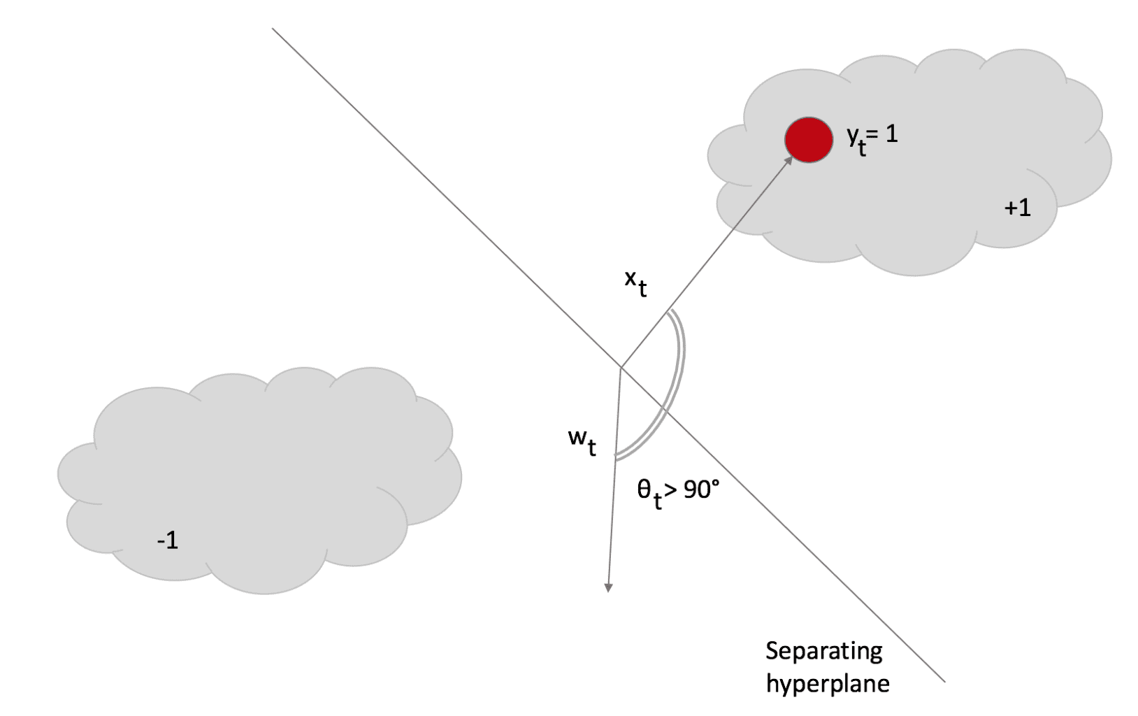
The angle θ > 90°; therefore, the dot product is negative, and the sample is classified as -1. However, its label is +1. In this case, the update rule becomes very aggressive because it looks for a new w, which must be as close as possible to the previous (otherwise, the existing knowledge is immediately lost). Still, it must satisfy L=0 (in other words, the classification must be correct).
The introduction of the slack variable allows soft margins (like in SVM) and a degree of tolerance controlled by parameter C. In particular, the loss function has to be L <= ξ, allowing a more significant error. Higher C values yield stronger aggressiveness (with a consequent higher risk of destabilization in the presence of noise), while lower values allow a better adaptation. This algorithm must cope with noisy samples (with wrong labels) when working online. Good robustness is necessary; otherwise, changes that are too rapid will produce higher misclassification rates.
After solving both update conditions, we get the closed-form update rule:

This rule confirms our expectations: the weight vector is updated with a factor whose sign is determined by y(t) and whose magnitude is proportional to the error. Note that if there’s no misclassification, the nominator becomes 0, so w(t+1) = w(t), while, in case of misclassification, w will rotate towards x(t) and stop with a loss L <= ξ. In the next figure, the effect has been marked to show the rotation. However, it’s usually as smallest as possible:
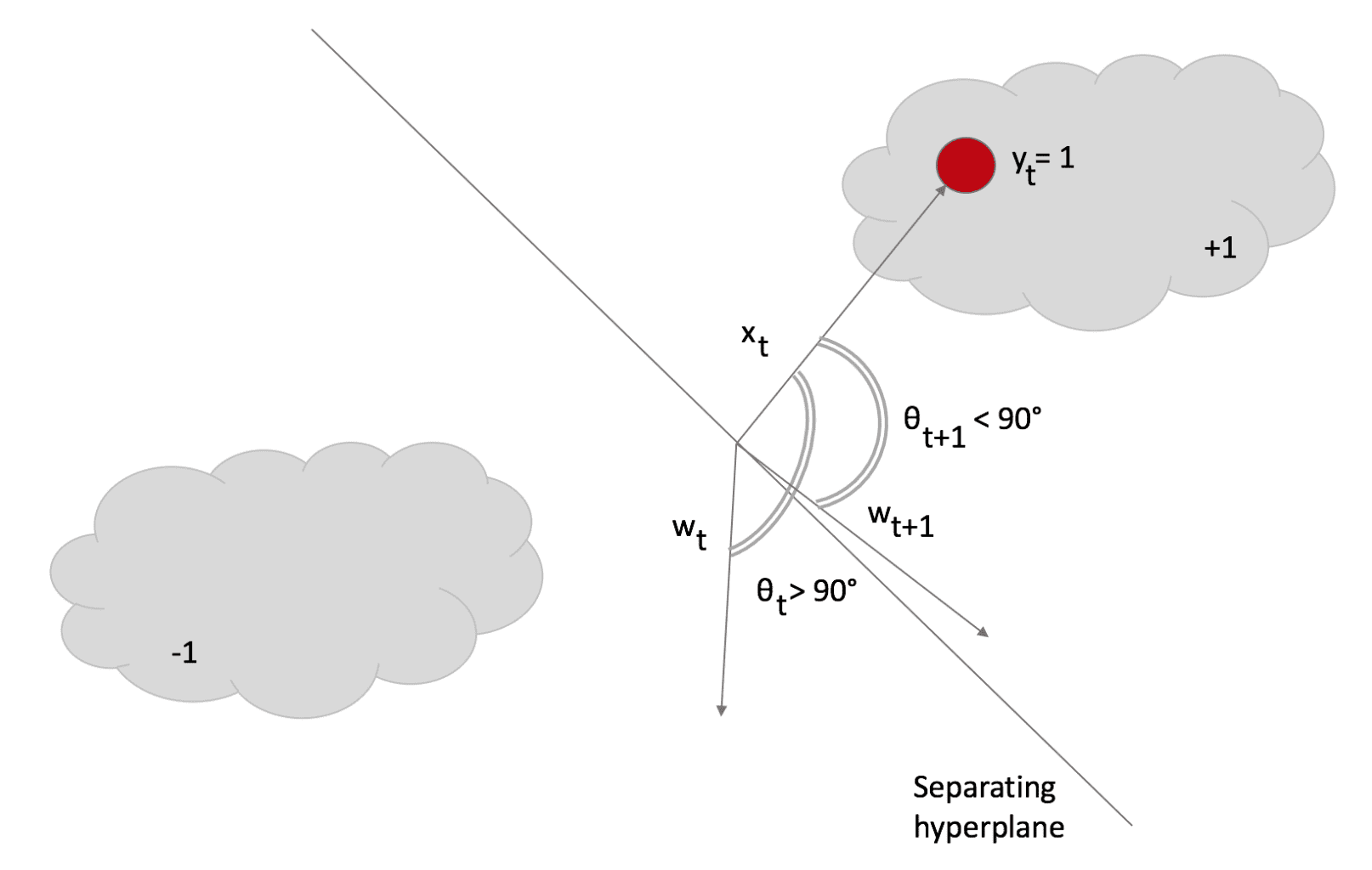
After the rotation, θ < 90° and the dot product becomes negative, so the sample is correctly classified as +1. Scikit-Learn implements Passive-aggressive algorithms, but I preferred implementing the code to show how simple they are. In the following snippet (also available in this GIST), I first create a dataset, then compute the score with a Logistic Regression, and finally apply the PA and measure the final score on a test set:
import numpy as np

from sklearn.datasets import make_classification
from sklearn.linear_model import LogisticRegression
from sklearn.model_selection import train_test_split

# Set random seed (for reproducibility)
np.random.seed(1000)

nb_samples = 5000
nb_features = 4

# Create the dataset
X, Y = make_classification(n_samples=nb_samples,
                           n_features=nb_features,
                           n_informative=nb_features - 2,
                           n_redundant=0,
                           n_repeated=0,
                           n_classes=2,
                           n_clusters_per_class=2)

# Split the dataset
X_train, X_test, Y_train, Y_test = train_test_split(X, Y, test_size=0.35, random_state=1000)

# Perform a logistic regression
lr = LogisticRegression()
lr.fit(X_train, Y_train)
print('Logistic Regression score: {}'.format(lr.score(X_test, Y_test)))

# Set the y=0 labels to -1
Y_train[Y_train==0] = -1
Y_test[Y_test==0] = -1

C = 0.01
w = np.zeros((nb_features, 1))

# Implement a Passive Aggressive Classification
for i in range(X_train.shape[0]):
    xi = X_train[i].reshape((nb_features, 1))

    loss = max(0, 1 - (Y_train[i] * np.dot(w.T, xi)))
    tau = loss / (np.power(np.linalg.norm(xi, ord=2), 2) + (1 / (2*C)))

    coeff = tau * Y_train[i]
    w += coeff * xi

# Compute accuracy
Y_pred = np.sign(np.dot(w.T, X_test.T))
c = np.count_nonzero(Y_pred - Y_test)

print('PA accuracy: {}'.format(1 - float(c) / X_test.shape[0]))
Regression
For regression, the algorithm is very similar, but it’s now based on a slightly different Hinge loss function (called ε-insensitive):

The parameter ε determines a tolerance for prediction errors. The update conditions are the same adopted for classification problems, and the resulting update rule is:

Just like for classification, Scikit-Learn also implements a Regression. However, in the next snippet (also available in this GIST), there’s a custom implementation:
import matplotlib.pyplot as plt
import numpy as np

from sklearn.datasets import make_regression

# Set random seed (for reproducibility)
np.random.seed(1000)

nb_samples = 500
nb_features = 4

# Create the dataset
X, Y = make_regression(n_samples=nb_samples,
                       n_features=nb_features)

# Implement a Passive Aggressive Regression
C = 0.01
eps = 0.1
w = np.zeros((X.shape[1], 1))
errors = []

for i in range(X.shape[0]):
    xi = X[i].reshape((X.shape[1], 1))
    yi = np.dot(w.T, xi)

    loss = max(0, np.abs(yi - Y[i]) - eps)

    tau = loss / (np.power(np.linalg.norm(xi, ord=2), 2) + (1 / (2*C)))

    coeff = tau * np.sign(Y[i] - yi)
    errors.append(np.abs(Y[i] - yi)[0, 0])

    w += coeff * xi

# Show the error plot
fig, ax = plt.subplots(figsize=(16, 8))

ax.plot(errors)
ax.set_xlabel('Time')
ax.set_ylabel('Error')
ax.set_title('Passive Aggressive Regression Absolute Error')
ax.grid()

plt.show()
The error plot is shown in the following figure:
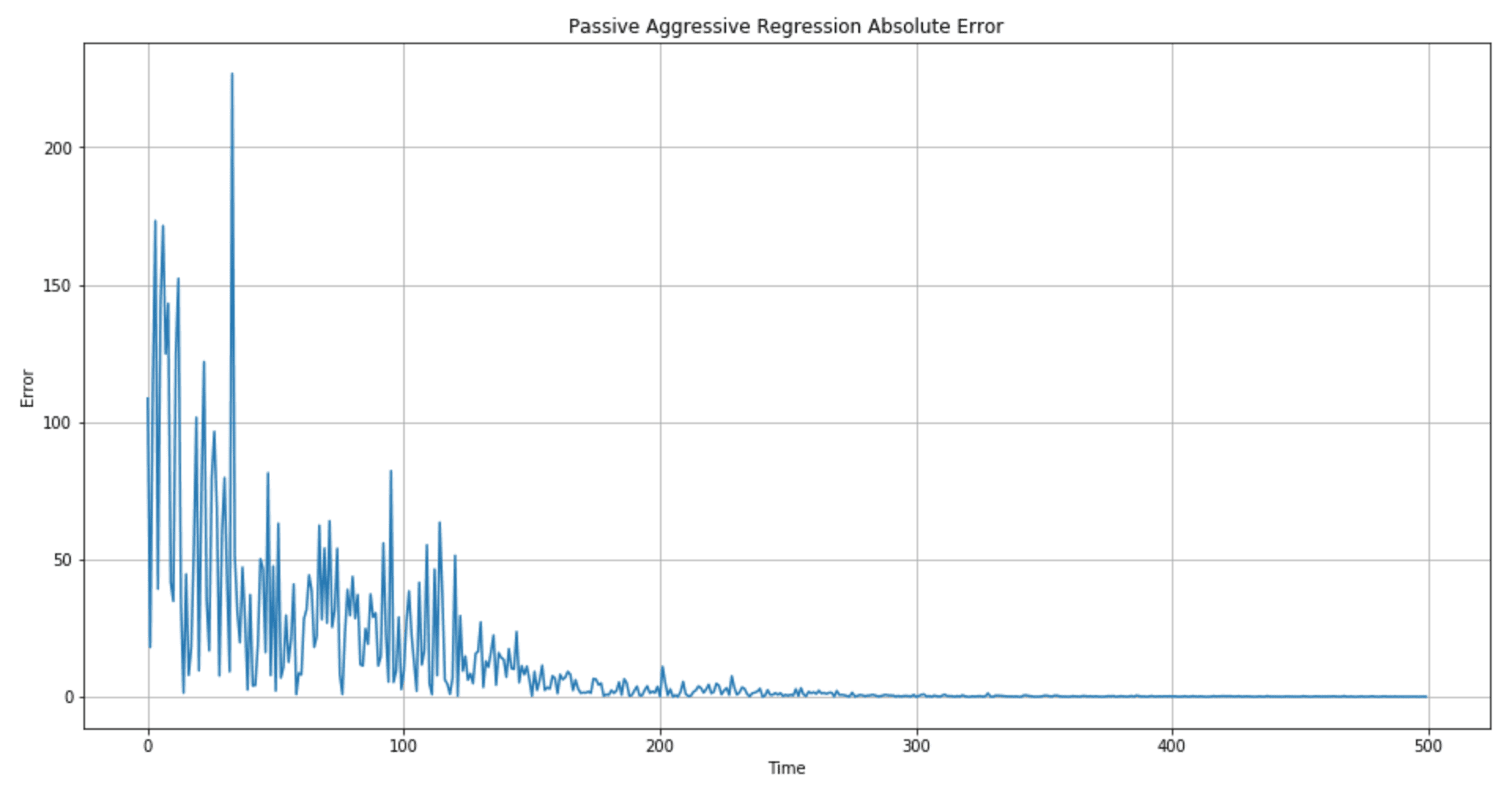
The regression quality (in particular, the length of the transient period when the error is high) can be controlled by picking better C and ε values. In particular, I suggest checking different range centers for C (100, 10, 1, 0.1, 0.01) to determine whether a higher aggressiveness is preferable.
References:
-
- Crammer K., Dekel O., Keshet J., Shalev-Shwartz S., Singer Y., Online Passive-Aggressive Algorithms, Journal of Machine Learning Research 7 (2006) 551–585
If you like this post, you can always donate to support my activity! One coffee is enough!