
Self-organizing maps (SOM) are neural structures proposed for the first time by the computer scientist T. Kohonen in the late 1980s (that’s why they are also known as Kohonen Networks). Their peculiarities are the ability to auto-cluster data according to the topological features of the samples and the approach to the learning process. Contrary to methods like Gaussian Mixtures or K-Means, a SOM learns through a competitive learning process. In other words, the model tries to specialize its neurons so as to be able to produce a response only for a particular pattern family (it can also be a single input sample representing a family, like a handwritten letter).
Let’s consider a dataset containing N p-dimensional samples. A suitable SOM is a matrix (other shapes, like toroids, are also possible) containing (K × L) receptors, each comprising p synaptic weights. The resulting structure is a tridimensional matrix W with a shape (K × L × p).
During the learning process, a sample x is drawn from the data generating distribution X, and a winning unit is computed as:

In the previous formula, I’ve adopted the vectorized notation. The process must compute the distance between x and all p-dimensional vectors W[i, j], determining the tuple (i, j) corresponding to the unit that has shown the maximum activation (minimum distance). A distance function must be computed once this winning unit has been found. Consider the schema shown in the following figure:
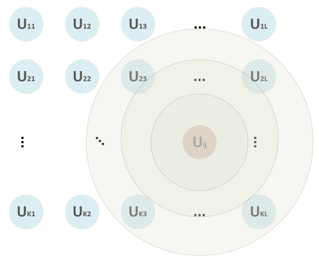
At the beginning of the training process, we are unsure if the winning unit will remain the same. Therefore, we apply the update to a neighborhood centered in (i, j) and a radius, which decreases proportionally to the training epoch. In the figure, for example, the winning unit can start also considering the units (2, 3) → (2, L), …, (K, 3) → (K, L), but, after some epochs, the radius becomes 1, considering only (i, j) without any other neighbor.
This function is represented as a (K × L) matrix whose generic element is:

The numerator of the exponential is the Euclidean distance between the winning unit and the generic receptor (i, j). The distance is controlled by the parameter σ(t), which should decrease (possibly exponentially) with the number of epochs. Many authors (like Floreano and Mattiussi, see the reference for further information) suggest introducing a time-constant τ and defining σ(t) as:

The competitive update rule for the weights is:

Where η(t) is the learning rate that can be fixed (for example η = 0.05) or exponentially decaying like σ(t), the weights are updated by summing the Δw term:

As it’s possible to see, the weights belonging to the neighborhood of the winning unit (determined by δf) are moved closer to x, while the others remain fixed (δf = 0). The role of the distance function is to impose a maximum update (which must produce the strongest response) in proximity to the winning unit and a decreasing one to all the other units. In the following figure, there’s a bi-dimensional representation of this process:

All the units with i < i-2 and i > i+2 are fixed. Therefore, when the distance function becomes narrow to include only the winning unit, a maximum selectivity principle is achieved through a competitive process. This strategy is necessary for the map to create responsive areas most efficiently. Without a distance function, the competition could not happen at all, or, in some cases, the same unit could be activated by the same patterns, driving the network to an infinite cycle.
Even if we don’t provide any proof, a Kohonen network trained using a decreasing distance function will converge to a stable state if the matrix (K × L) is large enough. I suggest trying smaller matrices (but with KL > N) and increasing the dimensions until the desired result is achieved. Unfortunately, however, the process is quite slow, and convergence is normally achieved after thousands of iterations of the whole dataset. For this reason, it’s often preferable to reduce the dimensionality (via PCA, Kernel-PCA, or NMF) and use a standard clustering algorithm.
An important element is the initialization of W. There are no best practices. However, if the weights are already close to the most significant components of the population, the convergence can be faster. A possibility is to perform a spectral decomposition (like in a PCA) to determine the principal eigenvector(s). However, when the dataset presents non-linearities, this process is almost useless. I suggest initializing the weights by randomly sampling the values from a uniform (min(X), max(X)) distribution (X is the input dataset). Another possibility is to try different initializations, computing the average error on the whole dataset and taking the values that minimize this error (it’s useful to try to sample from Gaussian and uniform distributions with a number of trials greater than 10). In general, sampling from a Uniform distribution produces average errors with a standard deviation < 0.1. Therefore, it doesn’t make sense to try too many combinations.
To test the SOM, I’ve used the first 100 faces from the Olivetti dataset (AT&T Laboratories Cambridge) provided by Scikit-Learn. Each sample is a length of 4096 floats [0, 1] (corresponding to 64 × 64 grayscale images). I’ve used a matrix with shape (20 × 20), 5000 iterations, using a distance function with σ(0) = 10 and τ = 400 for the first 100 iterations and fixing the values σ = 0.01 and η = 0.1 ÷ 0.5 for the remaining ones. In order to speed up the block computations, I’ve decided to use Cupy, which works like NumPy but exploits the GPU (it’s possible to switch to NumPy simply by changing the import and using the namespace np instead of cp). Unfortunately, there are many cycles, and it’s difficult to parallelize all the operations. The code is available in this GIST:
import cupy as cp
import matplotlib.pyplot as plt
import numpy as np

from sklearn.datasets import fetch_olivetti_faces

# Set random seed for reproducibility
np.random.seed(1000)
cp.random.seed(1000)

# Retrieve the dataset
faces = fetch_olivetti_faces()

nb_iterations = 5000
nb_startup_iterations = 100
nb_patterns = 100
pattern_length = faces['data'].shape[1]
pattern_width = pattern_height = int(np.sqrt(pattern_length))
eta0 = 1.0
sigma0 = 10
tau = 400.0
matrix_side = 20
precomputed_distances = np.zeros((matrix_side, matrix_side, matrix_side, matrix_side))

# Create the training set
X = faces['data']
X_train = cp.array(X[0:nb_patterns])

# Initialize the weights
W = cp.random.uniform(cp.min(X_train), cp.max(X_train), size=(matrix_side, matrix_side, pattern_length))

def winning_unit(xt):
    distances = cp.linalg.norm(W - xt, ord=2, axis=2)
    max_activation_unit = cp.argmax(distances)
    return int(cp.floor(max_activation_unit / matrix_side)), max_activation_unit % matrix_side

def eta(t):
    return eta0 * cp.exp(-float(t) / tau)

def sigma(t):
    return float(sigma0) * cp.exp(-float(t) / tau)

# Precompute the distances
for i in range(matrix_side):
    for j in range(matrix_side):
        for k in range(matrix_side):
            for t in range(matrix_side):
                precomputed_distances[i, j, k, t] = np.power(float(i) - float(k), 2) + np.power(float(j) - float(t), 2)

precomputed_distances = cp.array(precomputed_distances)

def distance_matrix(xt, yt, sigmat):
    dm = precomputed_distances[xt, yt, :, :]
    de = 2.0 * cp.power(sigmat, 2)
    return cp.exp(-dm / de)


if __name__ == '__main__':
  # Main cycle
  sequence = np.arange(0, nb_patterns)

  for t in range(nb_iterations):
      np.random.shuffle(sequence)

      if t < nb_startup_iterations:
          etat = eta(t)
          sigmat = sigma(t)
      else:
          etat = 0.1
          sigmat = 0.01

      for n in sequence:
          x_sample = X_train[n]

          xw, yw = winning_unit(x_sample)
          dm = distance_matrix(xw, yw, sigmat)

          dW = etat * cp.expand_dims(dm, axis=2) * (x_sample - W)
          W += dW

  # Show the weight matrix
  matrix_w = cp.zeros((matrix_side * pattern_height, matrix_side * pattern_width))

  for i in range(matrix_side):
      for j in range(matrix_side):
          matrix_w[i * pattern_height:i * pattern_height + pattern_height,
                   j * pattern_height:j * pattern_height + pattern_width] = W[i, j].reshape((pattern_height, pattern_width)) * 255.0

  fig, ax = plt.subplots(figsize=(12, 12))

  ax.matshow(matrix_w.tolist(), cmap='gray')
  ax.set_xticks([])
  ax.set_yticks([])

  plt.show()
The matrix with the weight vectors reshaped as square images (like the original samples) is shown in the following figure:

A sharp-eyed reader can see slight differences between the faces (in the eyes, nose, mouth, and brow). The most defined faces correspond to winning units, while the others are neighbors. Consider that each of them is a synaptic weight that must match a specific pattern. We can think of those vectors as pseudo-eigenfaces like in PCA, even if the competitive learning tries to find the values that minimize the Euclidean distance, so the objective is not to find independent components. As the dataset is limited to 100 samples, not all the face details have been included in the training set.
References:
-
- Floreano D., Mattiussi C., Bio-Inspired Artificial Intelligence: Theories, Methods, and Technologies, The MIT Press
If you like this post, you can always donate to support my activity! One coffee is enough!