

Keywords— customer journey, marketing, optimization, machine learning, reinforcement learning
Customer journeys as Markov Decision Processes
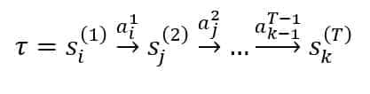
A static customer journey is often represented as a sequence of actions selected from a finite set A = {a1, a2, …, aN} where each element represents a specific marketing/commercial activity (e.g., F2F, e-mail, conference invitation, F2F follow-up, etc.). The sequence of actions can be statically designed according to predefined criteria, and an automatic system can suggest the next-best action according to the program. For example, a simple scenario can be based on the sequence:

Pause actions have been introduced to define a waiting time of at least two business days between two journey steps.
Therefore, the first action can be triggered by a CRM system, and after seven days, an automatic suggestion can be sent to the sales rep to invite her to arrange an F2F visit. Even if the process is straightforward, there are some evident drawbacks. First, every journey is an instance of a strictly defined class, which doesn’t consider any specific constraints (e.g., subjective reactions, preferences, etc.). Moreover, there’s no way to incorporate the feedback of an action into the flow, with the apparent consequence that all inappropriate actions will be repeated indefinitely.
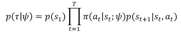
This paper analyzes an approach based on modeling the customer journey as a Markov Decision Process (MDP). This mathematical structure defines a sequential decision process that can be optimized so that a rational agent will always select the actions that maximize the expected final reward. We assume the environment is an abstract entity representing a specific context structured as discrete states S = {s1, s2, …, sM}. Analogously to actions, every state is associated with well-defined semantics (e.g., Customer visited twice) defined in every specific context. Considering the structure of a customer journey, it’s often helpful to define the states according to the actions, but this is not a necessary condition, and, in this paper, we are not going to impose such a constraint.
As the process is time-dependent, the evolution of the sequence of states (denoted using the Greek letter ) will be defined as:
This notation means that an agent started from the state s1 at t = 1 and ended in the state sK at t = T by selecting the actions indicated above the arrows. The choice of the discrete-time unit is arbitrary and not directly connected with the actual time flow. For example, a state can mean that an agent that has reached the state at t = a must wait for a predefined number of business days before taking another action. This choice allows to work in an asynchronous real-time scenario, which better describes the structure of an actual customer journey.
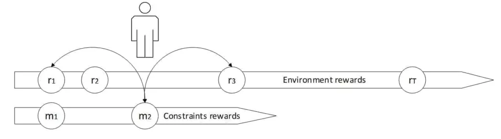
Another peculiarity of the environment is to provide feedback (from now on, we will call it reward) after each action the agent performs. Formally, the effect of an action performed by the agent is a transition from an origin state to a destination one [1]; therefore, we can define the quadruple SigmaJ:

The formula encodes the following steps:
-
- The agent is in the state Si at time t
- While in Si, the agent performs the action
- The agent receives the reward Rik, which is a real number, and if negative, it expresses a penalty (even if we are constantly referring to generic rewards)
- The environment transitions to the state Sj at time t+1
The sign of the reward indicates whether it’s positive or negative. At the same time, its absolute value is proportional to the level of goodness associated with the quadruple (e.g., r = 1 and r = -1 have the same magnitude – which can represent the impact predicted by the marketing department or subjectively perceived by the sales rep – but, while the former incentivizes the action, the latter penalizes it). It’s important to remember that a reward has no intrinsic meaning; instead, it must always be analyzed in the context of a state transition. The same action can yield different effects when the initial state changes (e.g., a first visit can have a positive reward, while an unwanted second one the day after might receive a negative reward).
A fundamental constraint that Reinforcement Learning requires is called exploring starts and implies that the agent can freely explore the whole environment in an infinite amount of time (i.e., all states are revisited an infinite amount of times). Such a condition is unrealistic because an honest sales rep cannot freely experiment with all possible strategies. However, our approximation assumes a sufficiently large number of existing journeys and, simultaneously, a limited number of possible states. Hence, on average, the agent can visit all states many times N >> Journey Average Length.
Uncertainty in the customer journeys
In the previous section, we defined a state sequence as a process where the actions trigger the transitions. This is generally correct, but we are not sure that an action will always lead to the same final state in real scenarios. Hence, it’s essential to introduce a more general structure that exploits the full expressivity of MDPs. We consider the sequence Tau:
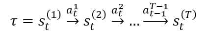
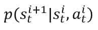
In this case, the state St(i) is a generic expression for “the state reached by the agent at time t = i.” Therefore, a single transition is associated with a conditional probability:
Such a probability has two essential features:
-
- It’s based on the Markov property. This means we don’t need to know history to predict a future state. It’s enough to consider only the previous state and the action that triggered the transition (this assumption is not always wholly realistic, but in most cases, such an approximation is reasonable and without negative consequences).
- It allows encoding multiple possible final states as a consequence of an action in an origin state.
In the remaining sections, we refer to stochastic processes, and our models always incorporate this uncertainty in the estimations. In customer journeys, the actions are always discrete. Therefore, the previous expression corresponds to a multi-dimensional associative array where each row contains the probabilities of every action. Suppose some scenarios are purely deterministic (i.e., an action in a state can trigger only a transition). In that case, it’s enough to set a single probability equal to 1 and all the remaining ones equal to 0 (e.g., a row will become equal to [0,0, …, 0,1,0, …, 0] where the one corresponds to the only possible action).
Rewards, Value, and Policies
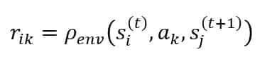
For our purposes, it’s helpful to introduce an appropriate notation to define all the remaining components of a customer journey. In the previous section, we have discussed the role of rewards. To keep the highest level of generality, we assume the existence of a function that outputs the reward corresponding to a transition:
Such a function can be explicitly modeled or considered part of the environment. In general, finding an approximation for RhoEnv is unnecessary because we’re only interested in the actual reward collected by the agent. However, for our calculations, it’s preferable to synthesize the reward sequence as a closed-form function.
Analogously to RhoEnv, we are going to introduce another function:
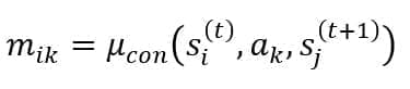
The values Mk are always rewards but are explicitly provided by a controlling agent (e.g., marketing or commercial department). They are aimed to impose specific constraints and encourage/discourage some actions artificially.
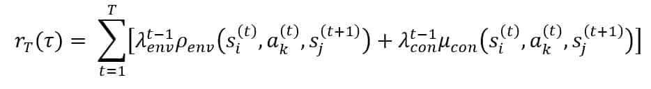
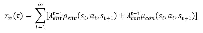
During a journey, the agent will collect a sequence of rewards, and its goal is to maximize the expected total reward. For this reason, we need to introduce a weighted sum of all rewards, assuming that at time t, the agent is interested in obtaining the most significant possible reward with a limited horizon. The sequence is unknown until completion, so we cannot assume perfect knowledge about the future. Hence, once in a state, the agent can either be guided to take the action that maximizes the immediate reward or an exponential decay sum of all the expected rewards over time. The latter choice is normally the best because it avoids premature choices and leads the agent to pursue the optimal result even if some intermediate actions are locally sub-optimal. Formally, we are going to express this concept by employing two discount factors, LambdaEnv and LambdaCon:
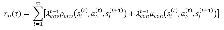
In the previous formula, we have implicitly supposed that the states s_i and s_j and the actions a_k refer to every single time value t. It’s easy to understand that the role of discount factors is to reduce the effect of future rewards. When λ_i→0, the horizon is limited to a single action, while λ_i→1 implies that all future actions have the same weight. Any choice in the range (0,1) allows for limiting the depth of the horizon. In our context, we are going to employ a value λ_env=0.75 and λ_con=0.15 because we want to limit the effect of the constraints to a single action and, at the same time, we prefer a model with a medium/long horizon to make always the best decisions concerning the final objective. Moreover, the previous sum is only theoretically valid because it never has infinite explorations. Therefore, in our calculations, we will truncate the sum to a limit T, representing the maximum length of the journeys.
In reinforcement learning, the agent decides according to a policy, which can be either deterministic or stochastic. A deterministic policy is a function that suggests the best action in every state. This is the most straightforward solution, but unfortunately, it’s not flexible enough to manage the uncertainty of real environments. That’s why we always refer to stochastic policies, which are, instead, conditional probability distributions Pi(Ak(t)|Sj(t)). The value output is a probability vector associated with every state. Once such information is available, the agent can either follow the policy (i.e., exploiting it by selecting the most probable action) or pick a random action (i.e., explore the environment and learn new elements). More formally, an action is chosen according to the following rule:
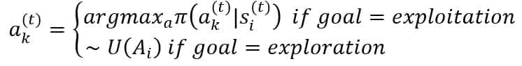
In the second case, the action is uniformly sampled from the set Ai of all possible actions in the state Si. Suppose the agent follows the policy Pi(Ak(t)|Sj(t)). In that case, the transition sequence will be obtained by multiplying the transition probabilities (encoding the uncertainty of the environment) by the policy value. However, as we will optimize only Pi, we always refer to it, omitting the transition probability. Therefore, considering the previous definition of discounted reward, an optimal stochastic policy is the one that maximizes the expected value of Rinf:
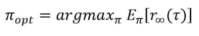
The research of an optimal policy is the goal of all reinforcement learning approaches. In the remaining part of the paper, we will discuss some strategies that can yield very positive results in the context of customer journeys. However, before moving forward, it’s helpful to introduce another explicit constraint, which is extremely important for regulatory reasons. The customer journeys must have a maximum fixed length T for a well-defined time window (e.g., a sales rep can visit a customer five times a year and must schedule her plan accordingly). This constraint is expressed by employing a truncated discounted reward:
This expression approximates the real discounted reward when T is large enough. The limit Lim LamdaK = 0 if K is in (0, 1) when t > T* as when the terms of the sum become negligible and for each Epsilon > 0 and Tau, there exists T > 0 so that the absolute value of |Rinf(Tau) – R*(Tau)| < Epsilon.
Environment models
In our context, the environment can be either standardized (e.g., when considering only micro-contexts) or highly variable. The latter option, however, is the most common for several reasons. The management of customer journeys is normally based on centralized brand strategies and, at the same time, on local regulations and directives. On the other hand, sales reps work in limited geographic areas, and their experience is often kept outside any modeling process. Our proposed strategy offers the advantage of keeping central control while actively collecting local feedback and adapting the journeys. For our simulations, we have implemented a neural model of the environments that can be represented as a parametrized function that outputs all the probabilities of all possible states after the agent has acted as the state St:
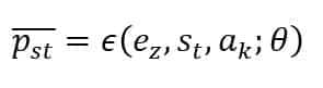
The function also accepts an indicator variable to switch between different environments (e.g., regions, counties, or micro-areas). Once the neural network has been trained using real customer journey data, such models can be employed to sample valid transition sequences and evaluate the rewards. Another approach we have employed is based on the observation that the states are discrete, and their number is generally very small. Therefore, it’s possible to estimate the transition matrices associated with each environment:

Every entry Pij represents the transition probability P(Si → Sj); hence, the sum of each row (each column) must always be equal to 1, and the single entries can be obtained through a frequency count. This method is more straightforward but not necessarily less effective, above all in those scenarios where there’s no need to model many environments. However, from our viewpoint, both approaches are equivalent because we are always assuming to work with a limited number of discrete states (clearly, a neural network can easily overcome this limitation, which instead is hard-coded in the transition matrices).
As discussed in the previous section, we will manage environment- and constraint-based rewards. The formers are supposed to be collected using an appropriate CRM application that must allow the sales rep to input her evaluation of the actions. The scale is always standardized and, in our case, corresponds to the range (-5, 5). Whenever possible, the feedback must be collected in an automated and, if necessary, anonymized way; for example, the evaluation of a conference can be obtained using an online survey and linked to the customer journey seamlessly. This choice limits the effect of the bias due to the natural desire not to report inadequate evaluations.
Even if the rewards represent a central element of our system, we will not create any model to predict them. Indeed, all the policies implicitly incorporate a substantial part of the reward dynamics. Still, considering the variability of such parameters, we think it’s not helpful to train a predictive model but rather to rely on quasi-real-time experiences to collect always the most accurate feedback. It’s also helpful to remember that a policy is a model that can be employed for a single sales rep or shared among a group of similar ones. Ideally, every single sales rep should be associated with her policy (that remains a time-variant model that is periodically retrained) to maximize the optimality and minimize the risk of generalized actions with limited applicability. Conversely, a large company could face the problem of training many models daily without any tangible advantage. In this context, we propose a strategy based on collaborative prototypes.
A set E of environments is initially selected according to geographical, political, and economic factors. Each sales rep is associated with a subset G, and her customer journey is randomly selected from the policies contained in G. All the collected feedbacks are averaged and employed to retrain the policies. After a cycle of n weeks, the set E is shuffled, and new subsets are selected and associated with the sales reps. Such a process is repeated for a fixed number of cycles or until the policies become stable (as they are time-variant, the stability must be measured and considered a maximum variation threshold). Once this process is concluded, a sales rep will be associated with the most compatible policy (i.e., the one whose best actions correspond to the most significant reported feedback). This method doesn’t offer the quality level of per-sales rep policies. Still, it minimizes the number of models and, at the same time, standardizes the customer journeys by classifying them into well-defined segments.
Customer Journey Optimization
The first policy search method is based on a classic approach [2] and [3]. It’s based on optimizing functions proportional to the expected reward obtained by averaging all possible customer journeys compatible with a specific context.
Consider an environment associated with a simplified version of the transition probability P(St+1|St, At) and a generic parametrized stochastic policy Pi(At|St; Psi). Both expressions are straightforward and use a single variable to indicate the evolution over time. We can model a generic transition sequence with a distribution that inherits the parameter vector Psi:
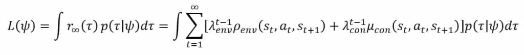
In the previous formula, p(S1) is the probability that Tau starts from S1. As the customer journeys often originate from the same initial state, it’s possible to set this value equal to 1 and omit the term. The discounted reward can be analogously simplified and rewritten as:
The expected value of the discounted reward is the function that we want to maximize:
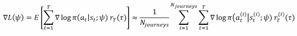
The best way to achieve the optimization is to perform a gradient ascent. Assuming T steps long transition sequences, it’s easy to prove the following result:
Further improvement can be obtained by employing methods like baseline subtraction [5], which yields a policy with a more minor variance. However, considering the low complexity of our environments, this optimization might now be required to achieve the desired accuracy.
An alternative method particularly suited for discrete environments is based on the Q-Learning algorithm [4] and [1]. Our goal is to model a state-action function Q(S(t), A(t)) that quantifies the advantage for an agent in the state St to pick an action instead of another. It’s easy to understand that an optimal policy is:
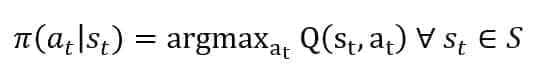
In this case, the agent will always select the action that maximizes the expected reward from a given state. The learning rule is self-explicative:
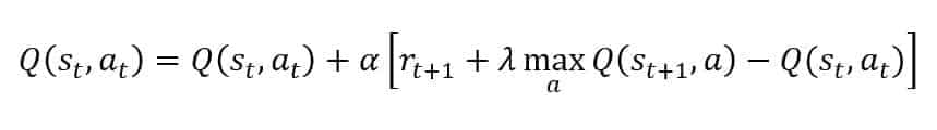
Once in a state, the agent will update the Q-value by considering the current reward Rt+1 and the maximum value[1] achievable by selecting the optimal action in the destination state St+1 (discounted by Lambda – in this way, a balance between immediate and future reward can be obtained). After a few iterations, the Q-function converges to a stable configuration representing the actual state-action mapping. The main advantage of this approach is its simplicity (there are only finite differences); moreover, the convergence is normally very fast given a sufficiently large number of exploring starts. As the agent is pushed to optimize the policy, the possible transition sequences will be limited without enough greedy exploration. This behavior is equivalent to accepting the first “best” result without considering any other alternative. Luckily, the number of states is generally small, and a concurrent activity of a group of sales reps is enough to collect a sample of valid transition sequences to bootstrap the first part of the training process.
However, as explained in the previous sections, any model-free reinforcement learning approach requires an exploration phase to avoid excluding large state-space regions from the policy. This behavior could not be entirely feasible when dealing with customer journeys because of the risk of losing potential customers. That’s why the model(s) must be trained with a real dataset, letting the agent explore alternatives only for a limited fraction of the total number of actions (e.g., contrary to the common practice, it’s possible to start with a percentage of 25% explorations, decreasing it monotonically until it reaches and maintains 0%). Alternatively, a valid strategy is to start every journey only with fixed exploitation sequences and to authorize the exploration only when the reward overcomes a predefined threshold. This method reduces the risk of premature, wrong actions and limits the analysis of alternative proposals only when the customer is engaged. The efficacy of such an approach is not comparable with an initial free exploration (that assumes an infinite number of episodes). Still, it has the additional advantage of allowing enforcing constraints from the beginning. Our simulation will show how this approach leads to a thorough exploration and complete modeling of the optimal policy given different starting states and contexts.
Simulation of Dynamic Optimization
To show the effectiveness of this approach, we have simulated 25,000 customer journeys[2] structured into six states:
-
- F2F call/interaction
- Email/Newsletter
- Webinar invitation
- Conference Invitation
- No action (Wait for 15 days before any other action)
- Success (Verified conversion) or Failure (Missed conversion)
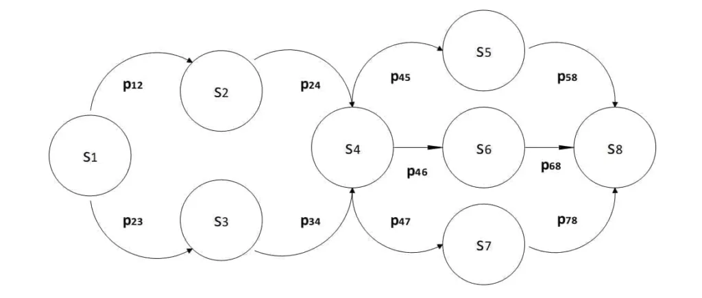
The maximum length of the customer journeys has been fixed to 10 steps, but, as we will see, most of them end after a smaller number of steps. To improve the visual result, we have structured the states in a matrix where each cell contains the state type, the final value, and the direction of the optimal transition. Such an organization can be visually pleasant, compact the states, and share part of the sequences among different journeys.
The agent is free to start from every cell, but in our experiments, we have imposed the constraint to start a customer journey always with an F2F call (which is a very realistic initial state in most cases). However, for completeness, the model has also been trained assuming a generic start from all the pause states (in particular, all those on the boundaries). The result of Q-Learning is shown in the following diagram. In this context, we want to consider some cases managed by the optimal policy.
-
- Pauses surround some boundary final cells (e.g. (4, 7)); therefore, analyzing them doesn’t make sense unless we are interested in immediate successes/failures.
- Starting from F2F, the algorithm has found several optimal strategies that are not immediate to verify. For example, at least two potential sequences are starting from (0, 0)
- F2F (0,0)→Pause (0,1)→Conference (1,1)→Webinar (2,1)→Pause(2,2)→Success
- F2F (0,0)→Pause (1,0)→Conference (1,1)→F2F (1,2)→Pause(2,2)→Success
- The difference between the two sequences is the action chosen after the invitation to a conference. Considering the expected rewards, the algorithm suggested inviting the customer to a webinar (e.g., for a more detailed follow-up). Still, the sales rep can achieve the same result with a F2F visit. The final state is a success in both cases. Still, in the latter, the final reward is smaller because it’s necessary to allocate a time slot, spending some time traveling, and the customer has less flexibility. If the goal of the visit is, for example, to confirm a hypothesis, a webinar can be much more efficient (both in terms of time and money). Therefore, the algorithm suggested such a policy.
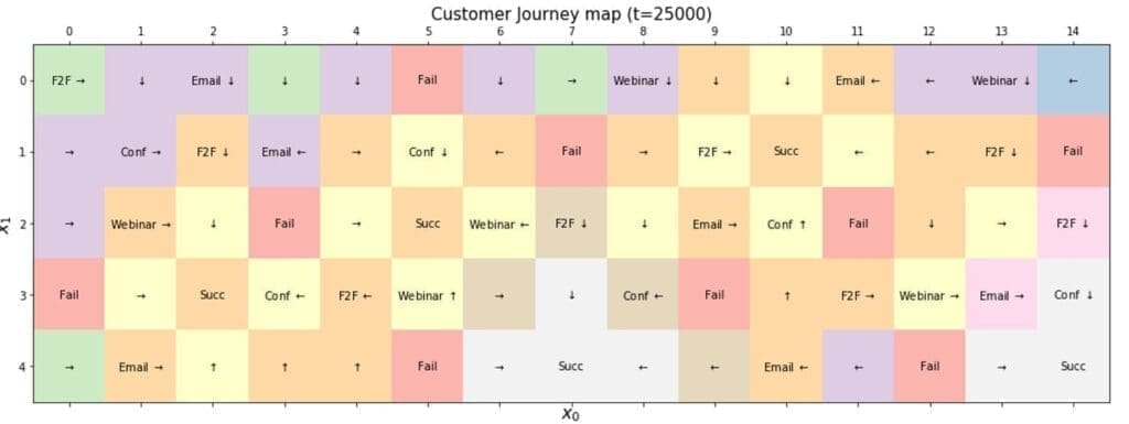
-
- When a virtual journey starts from a generic cell (excluding the terminal ones), it always reaches the success state that satisfies the double constraint Max(Reward) And Min(Path Length). Such a final state is often the closest to the starting because of the many journeys in the analysis. As discussed in the previous sections, collaborative training leverages different experiences to unify several journeys by merging the overlapping branches. For example, considering the starting states (1, 13) and (3, 11), they both end in the success state (4, 14) by sharing part of the transition sequences.
Conclusions And Further Developments
This post shows how applying standard reinforcement learning techniques to optimize a customer journey dynamically is possible.
References
-
- S. Sutton, A. G. Barto, Reinforcement Learning, Second Edition, A Bradford Book, 2018.
- J. Williams, Simple statistical gradient-following algorithms for connectionist reinforcement learning, Machine learning 8.3-4, 1992 pp 229-256.
- S. Sutton, et al. Policy gradient methods for reinforcement learning with function approximation, Advances in neural information processing systems. 2000.
- J. C. H. Watkins, P. Dayan, Q-Learning, Machine Learning, Kluwer Academic Publishers, May 1992, Volume 8, Issue 3–4, pp 279–292.
- Sugiyama, Statistical Reinforcement Learning: Modern Machine Learning Approaches, Chapman & Hall, 2015.
- Bonaccorso, Mastering Machine Learning Algorithms, Packt Publishing, Birmingham, 2018.
- Van Hasselt, A. Guez, D. Silver, Deep reinforcement learning with double q-learning, Thirtieth AAAI conference on artificial intelligence. 2016
- N. Lemon, P. C. Verhoef, Understanding customer experience throughout the customer journey, Journal of Marketing 80.6, 2016, pp 69-96
- Richardson, Using customer journey maps to improve customer experience, Harvard Business Review 15.1, 2010
- W. Wirtz, Multi-channel-marketing, Grundlagen–Instrumente–Prozesse, Wiesbaden, 2008
- S. Sutton et al., Policy gradient methods for reinforcement learning with function approximation, Advances in neural information processing systems, 2000
- Mnih et al., Asynchronous methods for deep reinforcement learning, International conference on machine learning, 2016.
Notes
[1] We haven’t explicitly introduced the concept of value in the context of reinforcement learning. However, for our purposes, it’s enough to say that the value of a state St is the expected reward obtainable by the agent by following a policy – possibly optimal – starting from St.
[2] For simplicity reasons, we haven’t included any real customer journey. All the data has been simulated, considering actual actions and expected reactions.
If you like this post, you can always donate to support my activity! One coffee is enough!